Case Report - Archives of Clinical and Experimental Surgery (2021)
A Case Study of the Application of WEKA Software to Solve the Problem of Liver Inflammation
Željko Đ Vujović*Željko Đ Vujović, Department of Electrical Engineering and Computer Science, University of Maribor, Montenegro, Europe, Email: etracon@t-com.me
Received: 16-Sep-2021 Published: 07-Oct-2021
Abstract
This paper aimed to consider the reliability of the basic metrics of evaluation of classification models: accuracy, sensitivity, specificity, and precision. The WEKA software tool was applied to the “Hepatitis C Virus (HCV) for Egyptian patient’s dataset”. The algorithms Bayesnet, Naivebayesh, Multilayer Perceptron, J48, and 10-fold crossvalidation were used in the study. The main results obtained are that, with all four algorithms in question, they achieved approximately the same accuracy of correctly classified specimens. BaiesNet-22.96%, Naïve Baies-26.14%, MultilaierPerceptron -26.57% and J48-25.27%. Binary classification metrics-sensitivity, specificity, and precision show very different values, depending on the intended class. Metric specificity, for all four algorithms, shows that a value that is in most of the range of possible values (0-1). Metric sensitivity and precision, for all four algorithms, showed values that are in the lower part of the range of possible values (0-1). The results of this study showed that WEKA software could not yet be considered as a relevant tool for the diagnosis of Hepatitis C Virus, on whose data set it was applied.
Introduction
This paper aimed to compare the properties of machine learning methods based on a decision tree, Support Vector Machine (SVM), neural networks, and Bayesian networks, with a specific example of a hepatitis C virus dataset for Egyptian patients. For this comparison, the reliability measures of the used algorithms were used: accuracy, sensitivity, specificity, and precision. The focus was on the classification model of WEKA software, developed at the University of Waikato, New Zealand, which, as one of the results, provides a detailed analysis of the accuracy of classifier predictions by class.
The reasoning behind this research was that it was not known what the accuracy, sensitivity, specificity, and precision of machine learning methods were based on a decision tree, machine support vector, neural networks, and Bayesian networks, which were theoretically addressed in work. The Big Data and Machine Learning which preceded this work [1-5].
The classification problem in WEKA software version 3.8.4 is solved by a variety of algorithms. The classifier directory contains a total of 56 algorithms, arranged in 7 folders, as follows: folder Bayes-6 algorithms, functions-11, lazy-3, meta-20, misk-2, rules-6, and trees-8. The decision tree used is the J48 algorithm [6-9]. For Machine Support Vector (SVM), there is an SMO algorithm in WEKA software. This algorithm was not used in the work because of the technical disadvantages of the machine on which the research was conducted. The Multilayer Perceptron algorithm was used for neural networks and Bayes Net and Naive Bayes for Bayesian networks [10-13].
The main results are that the accuracy of the four algorithms tested is approximately the same. It amounts to about 30%. This means that they did not prove to be good enough on the dataset to which they were applied [14-16]. This most likely indicates that new data is needed [17-20]. The possibility that a specific problem is not foreseeable has been ruled out for the time being. A possible reason for the weak traits shown by the algorithms used is that the data in the data set was not properly processed. The specificity metric is in the upper part of the range (0-1), which is its possible range of values. This means that the specificity is very good. In contrast, sensitivity and precision are in the lower range (0-1). This means that these metrics are not good enough. All of the above showed that the machine learning methods listed are not good enough under the conditions in which they were used [21- 28]. They also indicated that a possible direction for their improvement was the improvement of the preliminary processing of the data set that was analyzed and based on which the prediction was made, that is, the classification model was made. This enhancement of pre-processing includes scaling techniques, feature selection, data transformation, distribution transformation and data modeling [29,30]. A dataset that has 1385 instances is a small set. To solve the problem of predicting diseases caused by the hepatitis C virus, a larger data set is needed than the one discussed in this paper.
Case Presentation
Abstract
Egyptian patients who underwent treatment dosages for HCV about 18 months. Discretization should be applied based on expert recommendations; there is an attached file that shows how (Table 1).
| Data set characteristics | Attribute characteristics | Associated tasks | Number of instances | Number of attributes | Missing Values | Area | Date donated | Number of web hits |
|---|---|---|---|---|---|---|---|---|
| Multivariate | Integer, Real | Classification | 1385 | 29 | N/A | Life | 9/30/2019 | 32719 |
Source
Professor: Sanaa Kamal, (Professor of Medicine, Ain Shams University-Faculty of Medicine-Egypt), Prof. Dr. Khalid Abdelhameed ElBahnasy, (Professor of Information Systems, Faculty of Computer and Information Sciences, Ain Shams University-Egypt), Dr. Mohamed Hamdy ElEleimy, (Associate Professor at Information Systems Department, Faculty of Computer and Information Sciences, Ain Shams University- Egypt), Dr. Doaa Hegazy, (Assistant Professor at Information Systems Department, Faculty of Computer and Information Sciences, Ain Shams University- Egypt), Mr. Mahmoud Nasr, (MSc. Faculty of computer and information sciences-Ain Shams University- Egypt).
Confusion matrix for binary and four-class classification, TP Rate, FP Rate, Precision, Recall, F-Measure, Matthews Correlation Coefficient (MCC), Receiver Operating Characteristic Curve-ROC Area, Precision- Recall Curve Area - PRC Area. Confusion matrix for a binary classifier-Actual class values are labeled true (1) and False(0), and Predicted as Positive(1) and Negative(0). Performance estimates of classification models are derived from the terms TP, TN, FP, FN, existing in the confusion matrix (Table 2).
| Class | Actual class | ||
|---|---|---|---|
| Designation | True (1) | False (0) | |
| Predicted | Positive (1) | TP | FP |
| class | Negative (0) | FN | TN |
TP (True Positive)
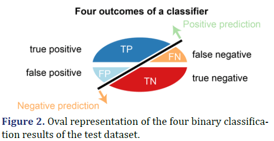
Data point in the confusion matrix is true positive when there is predicted a positive outcome and what happened is the same.
FP (False Positive)
Data point in the confusion matrix is false positive when there is a predicted positive outcome and what happened is a negative outcome. This scenario is known as Type 1 error. It is like a boon in a bad prediction.
FN (False Negative)
Data point in the confusion matrix is false negative when there is a predicted negative outcome and what happened is a positive outcome. This scenario is known as Type 2 error and it is considered as much dangerous as Type 1 error.
TN (True Negative)
Data point in the confusion matrix is true negative when there is predicted a negative outcome and what happened is the same.
Confusion matrix for four-class classification
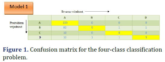
Four-class classification is a problem of classifying instances (examples) into four classes. Case of four classes: class A, class B, class C, and class D (Figures 1 and 2).
Accuracy
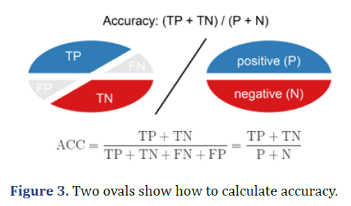
Accuracy is calculated as the total of two correct predictions (TP+TN) divided by the total number of data sets (P+N). The best accuracy is 1.0 and the worst is 0.0 (Figure 3).
Sensitivity (Recall or true positive rate-TPR)
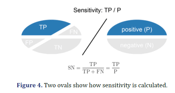
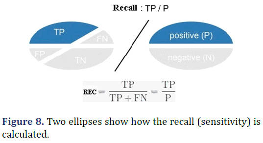
Sensitivity is calculated as the number of correct positive predictions (TP) divided by the total number of positive (P). Also called Recall (REC) or True Positive Rate. The best sensitivity is 1.0 and the worst is 0.0 ( Figure 4).
Specificity (True Negative Rate-TNR)
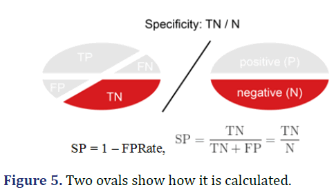
Specificity is calculated as the number of correct negative predictions (TN) divided by the total number of negatives (N). The best specificity is 1.0 and the worst is 0.0 (Figure 5).
False Positive Rate-FPR
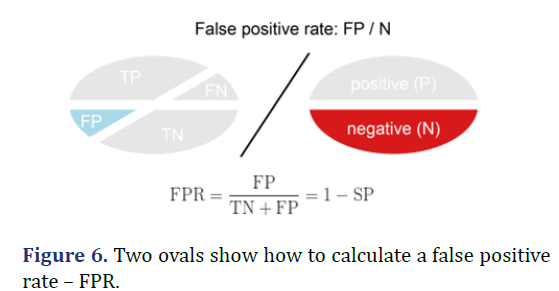
False Positive Rate is calculated as the number of False-positive Predictions (FP) divided by the total number of Negatives (N). The best False Positive Rate is 0.0 and the worst is 1.0. It can also be calculated as 1-specificity (Figure 6).
Precision
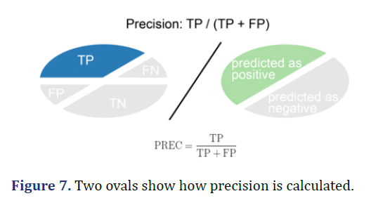
Precision is calculated as the number of correct positive predictions (TP) divided by the total number of positive predictions (TP+FP). The best precision is 1.0 and the worst is 0.0 (Figure 7).
Recall
F-measure: The F-score or F-measure is a measure of a test’s accuracy. It is calculated from the precision and recall of the test, where the precision is the number of true positive results divided by the number of all positive results, including those not identified correctly, and the recall is the number of true positive results divided by the number of all samples that should have been identified as positive. Precision is also known as a positive predictive value, and recall is also known as sensitivity in diagnostic binary classification (Figure 8).
F1-Score=2[precision*recall/(precision+recall)]
MCC: It’s a correlation between predicted classes and ground truth. It can be calculated based on values from the confusion matrix:
MCC=tp*tn-fp*fn/(tp+fp)tp+fn)(tn+fp)(tn+fn)
Alternatively, you could also calculate the correlation between y_true and y_pred. We can adjust the threshold to optimize MCC. When to use it, When working on imbalanced problems, When you want to have something easily interpretable.
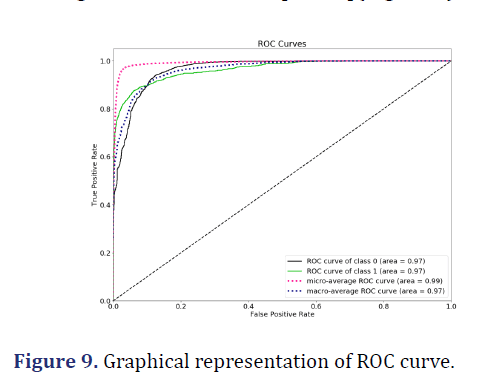
ROC area: It is a chart that visualizes the tradeoff between True Positive Rate (TPR) and False Positive Rate (FPR). Basically, for every threshold, we calculate TPR and FPR and plot them on one chart. Of course, the higher TPR and the lower FPR is for each threshold the better and so classifiers that have curves that are more top-left side are better. We can see a healthy ROC curve, pushed towards the top-left side both for positive and negative classes. It is not clear which one performs better across the board as with FPR<~0.15 positive class is higher and starting from FPR~0.15 the negative class is above [31-37](Figure 9).
ROC AUC score: To get one number that tells us how good our curve is, we can calculate the Area under the ROC Curve, or ROC AUC score. The more top-left your curve is the higher the area and hence the higher ROC AUC score.
Alternatively, it can be shown that the ROC AUC score is equivalent to calculating the rank correlation between predictions and targets. From an interpretation standpoint, it is more useful because it tells us that this metric shows how good at ranking predictions your model is. It tells you what is the probability that a randomly chosen positive instance is ranked higher than a randomly chosen negative instance [38- 41].
PRC area: The PRC Area is the area below the Precision- Recall curve. The PRC curve was obtained by combining precision (PPV) and sensitivity (TPR) for each threshold, the PPV and TPR are calculated and the corresponding graphe point is plotted (Figure 10).
PR AUC score/average precision: The Area under the Precision-Recall Curve is one number that describes model performance. PR AUC score is the average of precision scores calculated for each recall threshold (0.0, 1.0).
Results
Scheme 1
weka.classifiers.bayes.BayesNet-D-Q weka.classifiers. bayes.net.search.local.K2-- -P 1-S BAYES–ase E weka.classifiers.bayes.net.estimate. SimpleEstimator -- -A 0.5
Relation: HCV-Egy-Data_modified
Instances: 1385
Attributes: 29
Age, Gender, BMI, Fever, Nausea, Vomiting, Headache, Diarrhea, Fatigue and generalized bone ache, Jaundice, Epigastric pain, WBC, RBC, HGB, Plat, AST 1,ALT 1, ALT4, ALT 12, ALT 24, ALT 36, ALT 48, ALT after 24,RNA Base, RNA 4, RNA 12,RNA EOT,RNA EF, Baseline histological Grading, Baseline histological staging (Tables 1-15).
| Cross-validation | Results | |
|---|---|---|
| Correctly classified instances | 318 | 22.96% |
| Incorrectly classified instances | 1067 | 77.04% |
| Kappa statistic | -0.0287 | |
| Mean absolute error | 0.3763 | |
| Root mean squared error | 0.4393 | |
| Relative absolute error | 100.38% | |
| Root relative squared error | 101.48% | |
| Total number of instances | 1385 | |
| TP Rate | FP Rate | Precision | Recall | F-measure | MCC | ROC area | PRC area | Class |
|---|---|---|---|---|---|---|---|---|
| 0.107 | 0.186 | 0.156 | 0.107 | 0.127 | -0.091 | 0.423 | 0.205 | 1 |
| 0.271 | 0.27 | 0.241 | 0.271 | 0.255 | 0.001 | 0.51 | 0.249 | 2 |
| 0.214 | 0.266 | 0.217 | 0.214 | 0.216 | -0.052 | 0.457 | 0.234 | 3 |
| 0.32 | 0.307 | 0.27 | 0.32 | 0.293 | 0.013 | 0.524 | 0.281 | 4 |
| Weighted Avg. | ||||||||
| 0.23 | 0.258 | 0.222 | 0.23 | 0.224 | -0.032 | 0.479 | 0.243 |
| Scheme 1: Matrix | ||||
|---|---|---|---|---|
| a | b | c | d | |
| 36 | 94 | 94 | 112 | a=1 |
| 61 | 90 | 85 | 96 | b=2 |
| 79 | 94 | 76 | 106 | c=3 |
| 55 | 96 | 95 | 116 | d=4 |
| Cross-validation | Results | |
|---|---|---|
| Correctly classified instances | 362 | 26.14% |
| Incorrectly classified instances | 1023 | 73.86% |
| Kappa statistic | 0 | |
| Mean absolute error | 0.3748 | |
| Root mean squared error | 0.4329 | |
| Relative absolute error | 100.00% | |
| Root relative squared error | 100% | |
| Total number of instances | 1385 | |
| TP Rate | FP Rate | Precision | Recall | F-Measure | MCC | ROC area | PRC area | Class |
|---|---|---|---|---|---|---|---|---|
| 0 | 0 | ? | 0 | ? | ? | 0.496 | 0.241 | 1 |
| 0 | 0 | ? | 0 | ? | ? | 0.496 | 0.238 | 2 |
| 0 | 0 | ? | 0 | ? | ? | 0.496 | 0.255 | 3 |
| 1 | 1 | 0.261 | 1 | 0.414 | ? | 0.496 | 0.26 | 4 |
| Weighted Avg. | ||||||||
| 0.261 | 0.261 | ? | 0.261 | ? | ? | 0.496 | 0.249 |
| Scheme 2: Matrix | ||||
|---|---|---|---|---|
| a | b | c | d | |
| 0 | 0 | 0 | 336 | a=1 |
| 0 | 0 | 0 | 332 | b=2 |
| 0 | 0 | 0 | 355 | c=3 |
| 0 | 0 | 0 | 362 | d=4 |
| Cross-validation | Results | |
|---|---|---|
| Correctly classified instances | 368 | 26.57% |
| Incorrectly classified instances | 1017 | 73.43% |
| Kappa statistic | 0.0206 | |
| Mean absolute error | 0.3718 | |
| Root mean squared error | 0.5466 | |
| Relative absolute error | 99.20% | |
| Root relative squared error | 126% | |
| Total number of instances | 1385 | |
| TP Rate | FP Rate | Precision | Recall | F-measure | MCC | ROC area | PRC area | Class |
|---|---|---|---|---|---|---|---|---|
| 0.193 | 0.254 | 0.196 | 0.193 | 0.195 | -0.06 | 0.453 | 0.22 | 1 |
| 0.277 | 0.236 | 0.271 | 0.277 | 0.274 | 0.041 | 0.527 | 0.249 | 2 |
| 0.282 | 0.247 | 0.282 | 0.282 | 0.282 | 0.035 | 0.521 | 0.278 | 3 |
| 0.307 | 0.243 | 0.308 | 0.307 | 0.307 | 0.063 | 0.533 | 0.28 | 4 |
| Weighted Avg. | ||||||||
| 0.266 | 0.245 | 0.265 | 0.266 | 0.266 | 0.021 | 0.509 | 0.257 |
| Scheme 3: Matrix | ||||
|---|---|---|---|---|
| a | b | c | d | |
| 65 | 94 | 86 | 91 | a=1 |
| 79 | 92 | 86 | 75 | b=2 |
| 96 | 76 | 100 | 83 | c=3 |
| 91 | 78 | 82 | 111 | d=4 |
| Cross-Validation | Results | |
|---|---|---|
| Correctly classified instances | 350 | 25.27% |
| Incorrectly classified instances | 1035 | 74.73% |
| Kappa statistic | 0.0029 | |
| Mean absolute error | 0.3751 | |
| Root mean squared error | 0.5814 | |
| Relative absolute error | 100.07% | |
| Root relative squared error | 134% | |
| Total number of instances | 1385 | |
| TP Rate | FP Rate | Precision | Recall | F-measure | MCC | ROC area | PRC area | Class |
|---|---|---|---|---|---|---|---|---|
| 0.25 | 0.236 | 0.253 | 0.25 | 0.251 | 0.014 | 0.501 | 0.249 | 1 |
| 0.271 | 0.226 | 0.274 | 0.271 | 0.273 | 0.045 | 0.526 | 0.252 | 2 |
| 0.231 | 0.245 | 0.246 | 0.231 | 0.238 | -0.014 | 0.488 | 0.248 | 3 |
| 0.26 | 0.29 | 0.24 | 0.26 | 0.25 | -0.03 | 0.476 | 0.255 | 4 |
| Weighted Avg. | ||||||||
| 0.253 | 0.25 | 0.253 | 0.253 | 0.253 | 0.003 | 0.497 | 0.251 |
| Scheme 4: Matrix | ||||
|---|---|---|---|---|
| a | b | c | d | |
| 84 | 82 | 79 | 91 | a=1 |
| 67 | 90 | 80 | 95 | b=2 |
| 80 | 82 | 82 | 111 | c=3 |
| 101 | 74 | 93 | 94 | d=4 |
| Osjetljivost=TP rate | Specificnost=1-FP rate | Preciznost | ||||||||||
|---|---|---|---|---|---|---|---|---|---|---|---|---|
| Klasa | B.N. | N.B. | M.P. | J48 | B.N. | N.B. | M.P. | J48 | B.N. | N.B. | M.P. | J48 |
| Portalna fibroza (F1) | 0,107 | 0,000 | 0,193 | 0,250 | 0,814 | 1,000 | 0,746 | 0,764 | 0,156 | ? | 0,193 | 0,253 |
| Malo sepse (F2) | 0,271 | 0,000 | 0,277 | 0,271 | 0,790 | 1,000 | 0,746 | 0,774 | 0,241 | ? | 0.277 | 0.274 |
| Mnogo sepse (F3) | 0,214 | 0,000 | 0,282 | 0,231 | 0,734 | 1,000 | 0,753 | 0,754 | 0,217 | ? | 0,282 | 0,246 |
| Ciroza (F4) | 0,329 | 1,000 | 0,307 | 0,250 | 0,693 | 0,000 | 0,757 | 0,760 | 0,270 | 0,261 | 0,307 | 0,240 |
Accuracy=[BayesNet=22,96%, NaiveBayes=26,28%, MultilayerPerceptron=26,57%, J48=25,27%]
Test mode: 10-fold cross-validation
=== Classifier model (full training set) ===
Bayes Network Classifier
not using ADTree
#attributes=29 #classindex=28
Network structure (nodes followed by parents)
Age (1): Baselinehistological staging
Gender (1): Baselinehistological staging
BMI (1): Baselinehistological staging
Fever (1): Baselinehistological staging
Nausea/Vomting (1): Baselinehistological staging
Headache (1): Baselinehistological staging
Headache (1): Baselinehistological staging
Fatigue and generalized bone ache (1): Baselinehistological staging
Jaundice (1): Baselinehistological staging
Epigastric pain (1): Baselinehistological staging
WBC (1): Baselinehistological staging
RBC (1): Baselinehistological staging
HGB (1): Baselinehistological staging
Plat (1): Baselinehistological staging
== Stratified cross-validation ==
=== Summary ===
=== Detailed accuracy by class ===
=== Confusion matrix ===
=== Run information ===
Scheme 2
Weka classifiers.bayes.NaiveBayes
Relation: HCV-Egy-Data_modified
Instances: 1385
Attributes: 29
Age, Gender, BMI, Fever, Nausea,Vomting, Headache,- Diarrhea, Fatigue & generalized bone ache, Jaundice, Epigastric pain, WBC, RBC, HGB, Plat,AST 1, ALT 1, ALT4, ALT 12, ALT 24, ALT 36, ALT 48, ALT after 24,RNA Base, RNA 4,RNA 12,RNA EOT,RNA EF, Baseline histological Grading, Baseline histological staging.
Test mode: 10-fold cross-validation
=== Classifier model (full training set) ===
Naive Bayes Classifier
Class
Attribute 1 2 3 4
0.24) (0.24) (0.26) (0.26)
== Stratified cross-validation ===
=== Summary ===
=== Detailed accuracy by class ===
=== Confusion matrix ===
=== Run information ===
Scheme 3
Weka classifiers.functions.MultilayerPerceptron-L
0.3-M 0.2-N 500-V 0-S 0-E 20-H a
Relation: HCV-Egy-Data_modified
Instances: 1385
Attributes: 29
Age, Gender, BMI, Fever, Nausea, Vomting, Headache, Diarrhea, Fatigue & generalized bone ache, Jaundice, Epigastric pain, WBC, RBC, HGB, Plat, AST 1,ALT 1,ALT4, ALT 12,ALT 24 ALT 36,ALT 48,ALT after 24,RNA Base, RNA 4,RNA 12,RNA EOT,RNA EF, Baseline histological Grading, Baseline histological staging.;
Test mode: 10-fold cross-validation
=== Stratified cross-validation ===
=== Summary ===
=== Detailed accuracy by class ===
=== Confusion matrix ===
=== Run information ===
Scheme 4
weka.classifiers.trees.J48 -C 0.25 -M 2
Relation: HCV-Egy-Data_modified
Instances: 1385
Attributes: 29
Age, Gender, BMI, Fever, Nausea, Vomting, Headache, Diarrhea, Fatigue & generalized bone ache, Jaundice, Epigastric pain, WBC, RBC, HGB, Plat, AST 1,ALT 1,ALT4, ALT 12,ALT 24 ALT 36,ALT 48,ALT after 24,RNA Base, RNA 4,RNA 12,RNA EOT,RNA EF, Baseline histological Grading, Baseline histological staging.
Test mode: 10-fold cross-validation
Classifier model (full training set)
J48 pruned tree
===Stratified cross-validation ===
=== Summary ===
=== Detailed accuracy by class ===
=== Confusion matrix ===
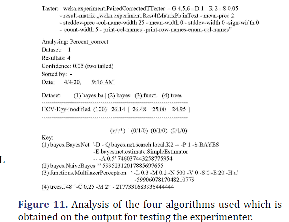
R1-comparison tables (Figure 11)
R2-support vector machine: Report on an attempt to execute the SMO algorithm
Not enough memory (less than 50 MB left on the heap). Please load a smaller dataset or use a larger heap size. Initial heap size 32 MB,
• Initial heap size 32 MB.
• Current memory (heap) used: 461.4 MB.
• Max memory (heap) available: 510 MB.
R3-rank and accuracy of algorithms
The experiment showed that all four algorithms used were of the same quality and that one of them could not be determined to be better than the rest. The Bayes Net algorithm showed an accuracy of 22.96%, Naïve Bayes 26.28%, Multilayer Perceptron 26.57%, and J48 25.
Discussion
A set of metrics is used to evaluate the classification model. The basic metrics, derived from the confusion matrix are TP; FP; FN, and TN. In addition following are used: ACC-Accuracy, ERP-Error Rate (1-ACC), TPRTrue Positive Rate, FPR-False Positive Rate, PREC-Precision (PPV-Positive Predictive Value), REC-Recall (TPR, Sensitivity), TNR-True Negative Rate (SP, Specificity), F-β score, MCC-Matthews Correlation Coefficient, ROC-Receiver Operating Characteristic Curve, PRC-Precision-Recall Curve and others.
In the results of this study, for all evaluated models, the following metrics were presented: TP Rate, FP Rate, Precision, Recall, F-Measure, MCC, ROC Area, PRC Area, and confusion matrix for four classes.
TP Rate-True Positive Rate is the same as the metall metric (Sensitivity) shows the sensitivity of the model to positive predictions shows the percentage of positive predictions, the probability that the actual positive value will be positive in medical diagnostics, for example, sensitivity the test is the ability of the test to correctly identify those who have the disease. It is a true positive rate. It shows how many positive labels the model has identified, of all possible labels.
FP Rate-False Positive Rate, a false positive rate (percentage, probability) is a measure of the accuracy of a test, whether it is a medical diagnostic test or something else. In technical terms, a false-positive rate is defined as the probability of falsely rejecting the null hypothesis.
Precision is the same as the PPV-Positive Predictive Value metric identifies the frequency at which the model was accurate in predicting positive class. This is the share of relevant copies among the downloaded copies. Unlike the Recall metric (sensitivity, reminder), which is the proportion of relevant copies that are downloaded.
The recall is the proportion of relevant cases found by a search, divided by the total number of existing relevant cases. Relevance indicates how well the downloaded document meets the user’s need for information. Relevance may include concerns such as timeliness, authority, or novelty of results.
The F-Measure or F-Score provides a combination of precision and sensitivity in one measure that captures both features, giving each the same weight. It is the harmonious middle of the two fractions, precision, and sensitivity. The result is a value between 0.0 for the worst F-measure and 1.0 for the perfect F-measure. A harmonic mean is defined as the reciprocal of the arithmetic mean of the reciprocal of a set of elements. In our case, we have two elements, precision (P) and sensitivity (R). Based on that, it was obtained that F-Measure=2 • (P • R) / (P+R). The F-Measure is interesting in some cases when more attention is paid to precision. For example, when false positives are more important to minimize, and false negatives are still important. In other cases, it is interesting when more attention is paid to sensitivity. For example, when false-negative results are more important to minimize, and false-positive results are still important.
The MCC-Matthews Correlation Coefficient takes into account the equilibrium ratio of the four categories of the confusion matrix (TP, FP, FN, TN). It is considered a balanced measure that can and should be used even when the classes are unbalanced. It is the basic correlation coefficient between the observed and the predicted binary classification. Name value from -1 to +1. A value of +1 represents a perfect prediction, 0-random prediction and -1 indicates a complete mismatch between prediction and observation. MCC is considered to be one of the best metrics for describing the confusion matrix of true and false positives and negatives by a single number. It does not depend on which class is positive.
ROC area is the area under the ROC curve (AUC). Summarizes the performance of each classifier in one measure and serves to compare classifiers. It is equivalent to the probability that a randomly selected positive instance is ranked higher than a randomly selected negative instance. AUC provides a unified measure of performance for all possible classification thresholds. AUC values range from 0 to 1. A model whose predictions are 100% incorrect has an AUC of 0.0, and one whose predictions are 100% correct has an AUC of 1.0. TPR and FPR are calculated for each threshold and plotted in a single graph. The higher the TPR and FPR for each threshold, the better. Based on this, it is concluded that better classifiers have more curves on the left. ROC AUC score is a number that corresponds to the area under the ROC curve. This indicator shows how good the model is in ranking predictions. It says what is needed: what is the probability that a randomly selected positive instance is ranked higher than a randomly selected negative instance. The ROC Area is higher, and thus the ROC AUC scores when the upper left curve is larger.
ROC curve (Receiver Operating Characteristic curve)
A ROC curve plots TPR vs. FPR at different classification thresholds. Lowering the classification threshold classifies more items as positive, thus increasing both False Positives and True Positives. The following figure shows a typical ROC curve. ROC curve is a graphical plot used to show the diagnostic ability of binary classifiers. A ROC curve is constructed by plotting the True Positive Rate (TPR) against the False Positive Rate (FPR). For example, in medical testing the true positive rate in which people are correctly identified to test positive for the disease in question. A discrete classifier that returns only the positive class gives a single point on the ROC space. But for probabilistic classifiers, which give a probability or score that reflects the degree to which give a probability or score that reflects the degree to which an instance belongs to one class rather than another, we can create a curve by varying the threshold for the score. Note that many discrete classifiers can be converted to a scoring classifier by ‘looking inside’ their instance statistics. For example, a decision tree determines the class of a leaf node from the proportion of instances at the node. The ROC curve shows the trade-off between sensitivity (or TPR) and specificity (1-FPR). Classifiers that give curves closer to the top-left corner indicate better performance. As a baseline, a random classifier is expected to give points lying along the diagonal (FPR=TPR). The closer the curve comes to the 45-degree diagonal of the ROC space, the less accurate the test is. Note that the ROC does not depend on the class distribution. This makes it useful for evaluating classifiers predicting rare events such as diseases or disasters. In contrast, evaluating performance using accuracy (TP+TN)/(TP+TN+FN+FP) would favor classifiers that always predict a negative outcome for rare events.
The Area Under the Curve (AUC)
To compare different classifiers, it can be useful to summarize the performance of each classifier into a single measure. One common approach is to calculate the area under the ROC curve, which is abbreviated to AUC. It is equivalent to the probability that a randomly chosen positive instance is ranked higher than a randomly chosen negative instance. A classifier with a high AUC can occasionally score worse in a specific region than another classifier with a lower AUC. But in practice, the AUC performs well as a general measure of predictive accuracy. AUC measures the entire two-dimensional area underneath the entire ROC curve (think integral calculus) from (0,0) to (1,1). AUC provides an aggregate measure of performance across all possible classification thresholds. One way of interpreting AUC is as the probability that the model ranks a random positive example more highly than a random negative example. AUC ranges in value from 0 to 1. A model whose predictions are 100% wrong has an AUC of 0.0; one whose predictions are 100% correct has an AUC of 1.0.
The PRC area is the area below the Precision-Recall curve. The PRC curve was obtained by combining precision (PPV) and sensitivity (TPR). For each threshold, the PPV and TPR and the corresponding gaffe point are calculated. Higher sensitivity means less precision. The sensitivity value, at which precision begins to decline rapidly, is used to select a threshold and a good model. By calculating the area under the precision-sensitivity curve, a number is obtained that describes the performance of the model. PR AUC is the average accuracy of the results for each sensitivity threshold [0.0;1.0]. The algorithm should have high precision and high sensitivity. These two metrics are not independent. That is why a compromise is made between them. A good PR curve has a higher AUC. Research has shown that PR is graphically more informative than ROC graphs when estimating binary classifiers on unbalanced sets.
Precision-recall curve
It is a curve that combines precision (PPV) and Recall (TPR) in a single visualization. For every threshold, you calculate PPV and TPR and plot it. The higher on the y-axis your curve is the better your model performance.
You can use this plot to make an educated decision when it comes to the classic precision/recall dilemma. Obviously, the higher the recall the lower the precision. Knowing at which recall your precision starts to fall fast can help you choose the threshold and deliver a better model.
We can see that for the negative class we maintain high precision and high recall almost throughout the entire range of thresholds. For the positive class, precision is starting to fall as soon as we are recalling 0.2 of true positives and by the time we hit 0.8, it decreases to around 0.7.
PR Curve is desired that the algorithm should have both high precision, and high recall. However, most machine learning algorithms often involve a trade-off between the two. A good PR curve has a greater AUC (area under the curve). In the figure above, the classifier corresponding to the blue line has better performance than the classifier corresponding to the green line. It is important to note that the classifier that has a higher AUC on the ROC curve will always have a higher AUC on the PR curve as well. Consider an algorithm that classifies whether or not a document belongs to the category “Sports” news. Assume there are 12 documents, with the following ground truth (actual) and classifier output class labels. By setting different thresholds, we get multiple such precision, recall pairs. By plotting multiple such P-R pairs with either value ranging from 0 to 1, we get a PR curve.
Consideration of experimental results
The Bayes Net, Naïve Bayes, Multilayer Perceptron, and J48 algorithms were used in the paper, four of the 56 algorithms embedded in WEKA software, because they were theoretically processed in the work that preceded this one. Algorithms solved the problem of four-class classification. Each instance of a classified data set could be assigned to one of four classes. 10- fold layered cross-validation was used to evaluate the model. This type of validation was chosen because it is widely known that it evaluates objectively the skill of a model, with little bias and little variance. Number 10 indicates the number of groups to which the data sample is divided. Each group has the same percentage of observations with a given categorical value. The general procedure of 10-fold cross-validation is performed as follows: The data set is shuffled randomly without hesitation; the mixed tax set is divided into 10 groups. For each group, individually, do the following: One group is taken as a hold-out set (test dataset). This set provides a final assessment of the model’s properties for machine learning, after training and model validation; the remaining groups are taken as a training dataset; the model is fitted with a training dataset and evaluated with a test dataset; the resulting model rating is retained and the model rejection. Modeling skills are summarized using a sample of model evaluation results.
Each observation in the data sample is assigned to an individual group and remains in that group for the duration of the procedure. Each sample is allowed to be used as the hold out set 1 time, and to train the model 9 times. An overview of the statistics for each algorithm compared shows how accurately the classifier could have predicted an instance class in the selected test mode. The values of the Kappa coefficients show that the observed algorithms are at the boundary between unacceptable and slightly acceptable quality. Mean absolute error and root mean squared error values may be considered satisfactory. High values of Relative absolute error and Root relative squared error indicate that the observed algorithms predict well.Detaljnu analizu tačnosti predviđanja po klasama, izražena je metrikama TP Rate, FP Rate, Precision, Recall, F-Measure, ROC Area i PRC Area. These metrics provide more information about the properties of the algorithms than the accuracy itself. Based on their values and definitions of sensitivity, specificity, and precision metrics, a table comparing the reliability parameters of the algorithms was made. It shows that the sensitivity, specificity, and precision of the algorithms are very different.
The values compared show the following hierarchy of algorithms accuracy: MultilayerPerceptron>Naive Bayes>J48>Bayes Net. Interestingly, the accuracy of correctly classified instances obtained by 10-fold cross-validation differs from the accuracy obtained by experiment using the Experimenter option. The reason for this difference could be the subject of special research.
The sensitivity hierarchy of algorithms for individual classes is, F1: J48>MultilayerPerceptron>- Bayes-Network>NaiveBayes, F2: MultilayerPerceptron> J48=BayesNetwork>NaiveBayesand, F3: Multilayer-Perceptron>J48>BN>NB, and for class F4: NaiveBayes>BayesNetwork>MultulayerPerceptron> J48. The Naive Bayes algorithm has poor sensitivity for all classes except class F4-Cirrhosis, for which it has the best sensitivity. It can be seen that the sensitivity values are in the lower part of the range (0,1), in which 0 is the worst sensitivity and 1 is the best. This means that the sensitivities could be better.
The hierarchy of specificity for individual classes is, F1: BayesNetwork>J48>MultilayerPerceptron> NaiveBayes, F2: BayesNetwork>- J48>MultilayerPerceptron>NaiveBayes, F3: J48>MultilayerPerceptron>BayesNetwork>Naive- Bayes, F4: J48>MultilayerPerceptron>-BayesNetwork> NaiveBayes. The table shows that specificity has values closer to the upper limit of the range (0,1), which contains values for specificity. This means that the specificity is very good. The precision hierarchy for individual classes is, F: J48>MultilayerPerceptron> Bayes-Network NaiveBayes, F1: MultilayerPerceptron> J48>BayesNetwork? NaiveBayes, F2: Multilayer- Perceptron>J48>BayesNetwork? NaiveBayes, F4: MultilayerPerceptron> BayesNetwork >Naive- Bayes >J48. The table shows that the precision values are closer to the lower limit of the range (0,1), which contains the precision values. He finds that precision could be better. The Confusion Matrix, at the output of the classifier, shows how many instances are assigned to each class. The elemental matrix shows the color of an example test whose real class is a row and the predicted class is a column.
Conclusions
This comparative analysis of the reliability metrics of machine learning algorithms, accuracy, sensitivity, specificity, and reliability showed:
- The observed algorithms have poor properties for classifying the data set in question. This can be seen from the accuracy values of each of these algorithms. The number of correctly classified examples is less than the number of incorrectly classified examples.
- Sensitivity, specificity and precision have, in com parison, very different values, which depend on the class being predicted. Specificity is very good and sensitivity and precision are satisfying. All this is not enough to conclude what kind of errors a classifier is making. Hepatitis C Virus (HCV) For Egyptian Patients Data Set should be increased, so that it can be used as a reliable basis for modeling and predicting diseases caused by the hepatitis C virus.
- A new, larger data set needs to be pre-processed, which includes scaling techniques, feature selection, data transformation, distribution transformation and data modeling. In particular, other metrics for evaluating classification models need to be studied, primarly F-Measure, MCC, ROC Area, PRC Area.
- A new, larger data set needs to be pre-processed, which includes scaling techniques, feature selection, data transformation, distribution transformation and data modeling. In particular, other metrics for evaluating classification models need to be studied, primarly F-Measure, MCC, ROC Area, PRC Area.
Author’s contribution
The conception, design, acquisition, analysis, and interpretation of data are on the whole based on the contribution of the author. This is, on the whole, individual research work. The author agrees that issues related to the accuracy or integrity of any part, even those in which the author is not personally involved, should be investigated and resolved and the resolution documented in the literature.
Acknowledgements
Not applicable.
Availability of Data and Materials
All data generated or analyzed during this study are included in this published article [and its supplementary files].
Competing Interests
The author declares that he has no, financial competing interests. The author declares that he has no known non-financial competitive interests.
Funding
Not applicable
References
- Nissim N, Shahar Y, Elovici Y, Hripcsak G, Moscovitch R. Inter-laborer and intra-labeler variability of condition severity classification models using active and passive learning methods. Artif Intell Med 2017;81:12-32.
- Ren W, Sun BQ, Tang H, Huang J, Lin H. Identify and analysis crotonylation sites in histone by using support vector machine. Artif Intell Med 2017;83:75-81.
- Wei L, Guo S, Kalvin KL Wong. A novel hierarchical selective ensemble classifier with bioinformatics applications. Artif Intell Med 2017;83:82-90
- Ž.Vujović. The big data and machine learning. J Inf Technol 2020;19:11-19.
- https://machinelearningmastery.com/load-csv-machine-learning-data-in-weka, Jan.23,2016.(Pr.01.03.20)
- Nandakumar S. Confusion matrix-are you confused? (Part I and Part II). Towards Data Science. 2020
- Brownlee J. How to work through a binary classification project in weka step-by-step. Machine learning mastery
- Sunasra M. Performance metrics for classification problems in machine learning. Medium. 2017
- Kumar A. ML Metrics: Sensitivity vs. Specificity. D Zone. 2018
- Maklin C. Metrics for evaluating machine learning classification models. Towards data science. 2019
- Brownlee J. Design and run your first experiment in weka. Machine learning mastery. 2019.
- Remco R. Bouckaert .WEKA manual for version 3-7-8.University of Waikato. 2013.
- Dua D, Graff C.UCI machine learning repository irvine, CA: the University of California. School of information and computer science. 2019.
- Liu X. A discretization algorithm based on a heterogeneity criterion.IEEE.2005
- Brownlee J. What is a confusion matrix in machine learning. Machine learning mastery.2020.
- Novaković JĐ. Solving machine learning classification problems, Rešavanje klasifikacionih problema mašinskog učenja. Fakultet tehničkih nauka u Čačku.2013
- Purva Huilgol. Accuracy vs. F1-Score.Analytics vidhya.2019
- Bouckaert RR, Frank E, Hall M, Kirkby R, Reutermann P, Sewald A, et al., WEKA manual for version 3-7-8. University of Waikato,2013
- https://classeval.wordpress.com/introduction/basic-evaluation-measures/ Dec.20,16.
- Nasr M.A novel model based on non invasive methods for prediction of liver fibrosis. IEEE.2019
- Brownlee J. What is a confusion matrix in machine learning. Machine learning mastery.2020.
- Jason Brownlee. A gentle introduction to k-fold cross-validation. Machine learning mastery .2018
- Charman Chan. What is a ROC curve and how to interpret it. DISPLAYR .2021.
- Saito T, Rechmsmeier M. The precision-recall plot is more informative than the ROC plot when evaluating binary classifiers on imbalanced datasets. Plos one 2015;10:3
- Euklend S.Precision-recall curves-what are they and how are they used. Acute care testing.2017
- Uberoi A. Precision-recall curve|ML , Last Updated: 19. Jul 2019.https://www.geeksforgeeks.org/precision-recall-curve-ml/ (Accessed, 18.04.2021.)
- Vujović Đ.Ž. Classification model evaluation metrics. Int J Adv 2021; 12: 6
- Iqbal A, Aftab S , Ali U , Nawaz Z, Sana L , Ahmad M , et al .Performance analysis of machine learning techniques on software defect prediction using nasa datasets . Int J Adv 2019;10: 5
- Alshammari M, Mezher M. A comparative analysis of data mining techniques on breast cancer diagnosis data using weka toolbox. Int J Adv 2020;11: 8
- Ayyagari M. Classification of imbalanced datasets using one-class svm, k-nearest neighbors and cart algorithm. Int J Adv 2020;11: 11
- Albahr A, Albahar M. An empirical comparison of fake news detection using different machine learning algorithms .Int J Adv 2020;11: 9
- Huapaya HD, Rodriguez C, Esenarro D. Comparative analysis of supervised machine learning algorithms for heart disease detection. Glosses of innovation applied to SMEs. 2020.
- Fawcett T. ROC graphs: Notes and practical considerations for researchers .Kluwer academic publishers. 2003.
- Tharwat A. Classification assesment methods. Appl. Comput 2020; 17:1
- Khan B, Shukla PK, Ahirwar MK . Strategic analysis in prediction of liver disease using different classification algorithms . Int j eng 2019; 7(7): 71-76
- Singh, Jagdeep, Bagga, Sachin, Kaur, Ranjodh. Software-based prediction of liver disease with feature selection and classification techniques. Procedia Comput Sci 2020; 167: 1970-1980
- Chicco D, Tötsch N, Jurman G .The Matthews Correlation Coefficient (MCC) is more reliable than BioDataMining balanced accuracy .BioData Min 2021; 13(1)
- Chicco D, Jurman G. The advantages of the Matthews Correlation Coefficient (MCC) over F1 score and accuracy in binary classification evaluation. BMC Genomics 2020 ;21(1):6.
- Singh S.How I achieved RMSLE = 0.43 in mercari price suggestion kaggle challenge . Medium .2019.
- Brownlee J.A gentle introduction to imbalanced classification . Machine learning mastery .2019
- Pankaj Malhotra .What is an imbalanced dataset?. Quora.2015.


